How I built Mindscape Explorer
I have listened to Sean Carroll’s Mindscape since it started in 2018, and for most of that time I have had a question about it that no single episode could answer. The show is built on breadth. A physicist interviews biologists, economists, philosophers, novelists, and political scientists, with solo lectures and listener-question episodes in between. I wanted to know what that breadth looks like when the whole archive is treated as one body of text. Which subjects does the show keep returning to? Which pairs of subjects have never shared an episode? Does a prepared lecture move through its material differently from a conversation? And could I search all of it by what I meant instead of by the words I happened to remember?
This post is the record of how I went about answering those questions. The result is Mindscape Explorer, and a companion page that checks whether a listener question has already been asked. I want to be upfront that I built both with Claude as a collaborator. The code was written in conversation and run on my own machine, every number below came off that machine, and the evaluation decided what shipped.
For anyone who wants the results without the story, they are these. Topic models fit without seeing Sean’s hand-assigned subject tags predict those tags at a macro average precision of 0.649, against 0.549 for a classifier that sees every word and 0.078 for chance. Solo lectures wander through topic space as much as interviews do (a difference of medians of −0.42 with an interval that spans zero), and the AMAs wander nearly twice as far. A serendipity recommender is twice as varied as the obvious “more like this” list (+0.33 in intra-list diversity, interval 0.32 to 0.34) at no measurable cost in novelty. A second, embedding-based representation agrees with the word-count one at a Mantel correlation of 0.644. The search reranker keeps 99% of its full result set at a 12-second budget, and the companion question-checker finds the right prior question first on 98% of paraphrases. The rest of the post says how each of those was measured.
Getting the transcripts without being a nuisance
Sean publishes a full transcript with every episode, embedded in the WordPress post behind a “show transcript” toggle. So I never had to fetch the episode pages themselves. WordPress exposes a JSON API, and paging through it pulls every post in twenty or thirty requests. The scraper checks robots.txt before each request, identifies itself with a user agent that carries my email address, waits three seconds between calls, honors Retry-After on rate limits, and caches every raw response to disk so that a parser change never causes a second fetch. The first run took about two minutes, most of it deliberate waiting, and the scraper has touched the live site only a handful of times since. New episodes land on the last cached page, so an update costs a few requests.
The parsing was the harder part. Across eight years the transcripts use five different conventions for marking speakers and timestamps, and I had to survey the archive to find all five. I held to one rule, which is that nothing is dropped silently. Of 444 posts, 439 have transcripts and 436 parse into labeled utterances. The 5 without transcripts have none on the site (a welcome post, two holiday messages, an AMA whose audio was Patreon-only, and a link to an outside interview), and the 3 that were published without speaker labels carry a flag and null speakers instead of a guess. A future episode in a sixth convention would show up as a flagged row for me to extend the parser against. The corpus is 7.4 million words of transcript.
A pipeline that knows what changed
The analysis grew to sixteen stages, and early on I lost a day to a chart rendered from a stale intermediate file. So the runner became a small make. Each stage writes a manifest that records a fingerprint of the corpus, a hash of the stage’s own source, its parameters, and the vintages of its upstream stages, and a stage runs only when one of those has changed. A re-scrape rebuilds everything, an edit to one module rebuilds that stage and its dependents, and a run with nothing changed does nothing. The website is the final stage, so the published page can never lag the analysis. This is unglamorous work, and it is the reason every number on the site and in this post agrees with every other.
Deciding how many topics there are
The core representation is a topic model. TF-IDF over one- to three-word terms (the show’s vocabulary is multi-word, and “dark matter” or “wave function” is a single idea) is factored by non-negative matrix factorization. Every topic model has to answer how many topics there are, and I did not want to pick the number by hand. The pipeline sweeps k and records three curves, for topic coherence, stability across random restarts, and reconstruction error. Coherence alone rises with k without limit, so its maximum only tells you where the grid ends. The combined score of coherence and stability has a real peak, but the bare maximum turned out to be sensitive to noise. When two episodes were added in September it flipped from 20 topics to 50. So the selection uses the one-standard-error rule from the tree-pruning and clustering literature. The restarts the sweep already runs give each k a standard error, and the smallest k within one standard error of the best score wins. Candidates within the noise count as ties, and ties break toward the simpler model.
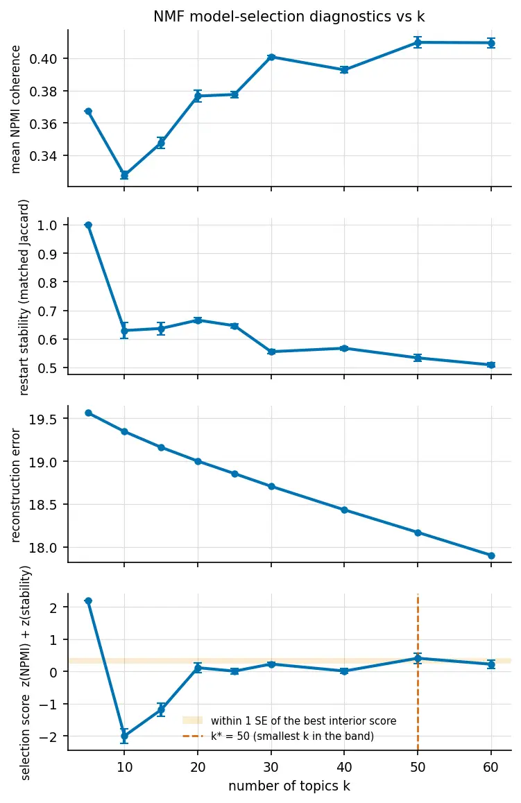
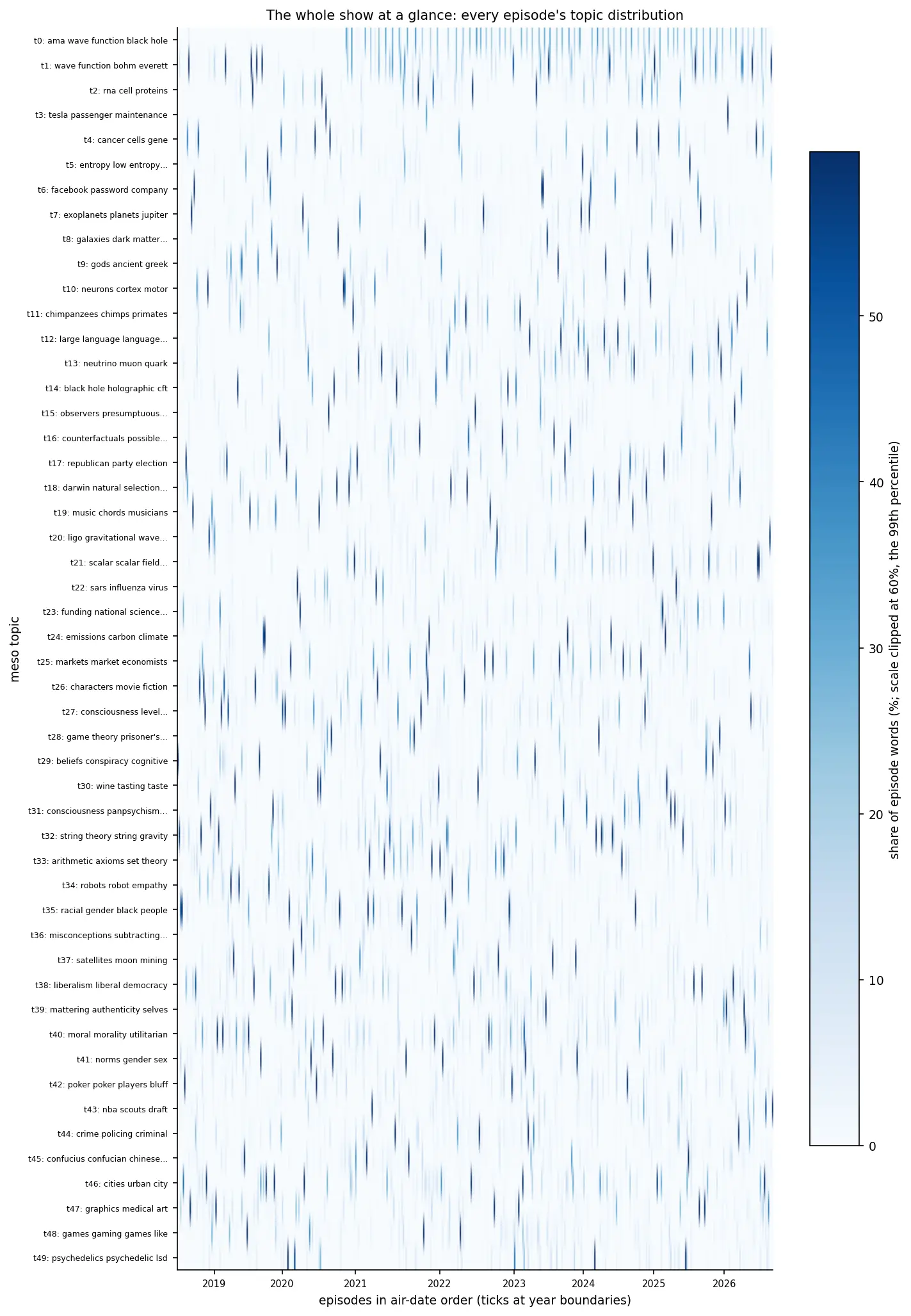
That gives an anchor of 50 topics. The site then works at three resolutions, 27, 50, and 92. The step between them is a fixed ratio of about 1.84 inherited from the larger project this grew out of, which uses one scale step everywhere rather than tuning a new one per analysis (for the curious, it is the tribonacci constant), so the coarse and fine resolutions are the anchor divided and multiplied by it. Whether the coarse topics contain the fine ones is inspected rather than assumed. The pipeline writes the similarity matrix between adjacent resolutions and a best-parent table for every fine topic.
Checking the model against the person who made the show
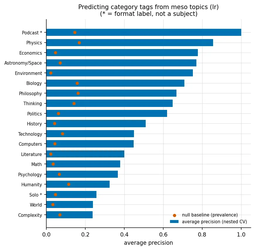
A topic model can always be read into. The check I trusted most was one the model had no part in. Sean assigns each episode a handful of subject tags by hand, and the topics were fit without ever seeing them. If the topics are real, they should predict the tags. So the pipeline trains one classifier per tag on each feature set and scores it by nested cross-validation, so that no score ever touches the data used to tune it, with format tags like “Podcast” and “Solo” excluded from the average.
Reading only the topic loadings, a gradient-boosted model predicts Sean’s 17 subject tags at a macro average precision of 0.649, against a chance level of 0.078. A logistic regression on the full TF-IDF matrix, which sees every word, scores 0.549, so the topics carry more of the tagging signal than the raw words do. The per-tag results are the more interesting reading. Physics, Biology, Astronomy, Economics, and Environment have vocabularies of their own and come back at 0.81 to 0.90. Humanity, World, and Psychology barely beat chance, at 0.37 to 0.42, and I think that is the right answer. Those tags record an editorial judgment about what an episode is for, and no count of words is going to carry that.
The finding I got wrong in advance
I expected a prepared solo lecture to move in a straight line through its subject and a conversation to ramble. To test that, every transcript is cut into tenths, each tenth is projected onto the fixed topic basis by non-negative least squares, and the route an episode walks through topic space is the sum of Hellinger steps between consecutive tenths. Solo lectures have a median route of 3.12 (95% bootstrap interval 2.66 to 3.90, n = 28) and interviews 3.54 (3.38 to 3.74, n = 347). The difference of medians is −0.42, with an interval from −0.90 to +0.44 and a permutation p of 0.22, so the two formats cannot be told apart. The episodes that wander are the AMAs, at 6.44 (6.34 to 6.63, n = 64), which is 2.91 further than an interview (2.66 to 3.16, p < 0.001), because each one answers dozens of unrelated listener questions in a single sitting.
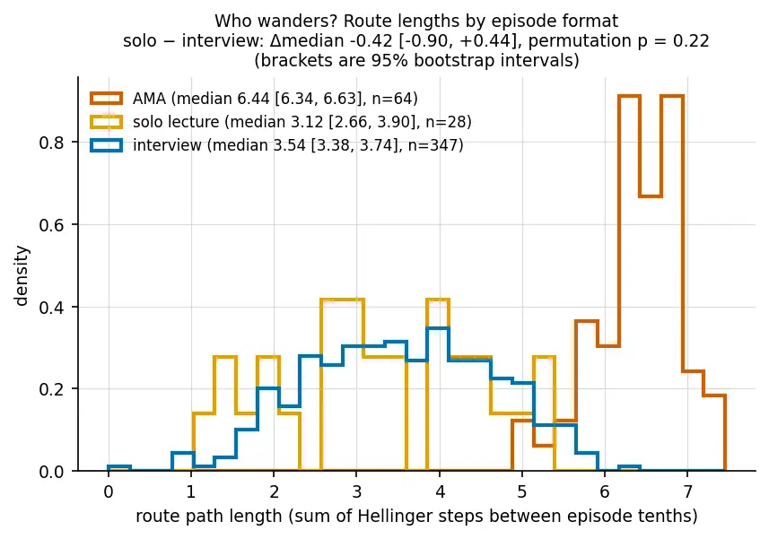
There is a second half to this that I would have missed with only one representation. Measured again in sentence-embedding space (more on that below), the three formats walk similar distances. AMAs have a median route of 2.14 (2.07 to 2.21), solo lectures 2.19 (2.01 to 2.41), and interviews 2.36 (2.32 to 2.39), and the rank correlation between the lexical routes and the semantic ones is 0.04. An AMA changes its words far more than it changes its meaning, which is what you would expect from a host answering physics questions in a physicist’s vocabulary all afternoon.
A recommender scored on more than accuracy
There is no listening data here, so relevance has to mean topical affinity, measured as the Bhattacharyya coefficient between two episodes’ topic distributions and averaged over the three resolutions. Each episode gets three lists. The first is the obvious “more like this”. The second is a serendipity list in the sense of Ge and colleagues. It must clear a relevance floor and it excludes the accuracy top-N, but it is ranked by the affinity carried through the seed episode’s minor topics, with the bridging topic reported, and then spread out by maximal marginal relevance. The third is a deliberate “least likely from here”.
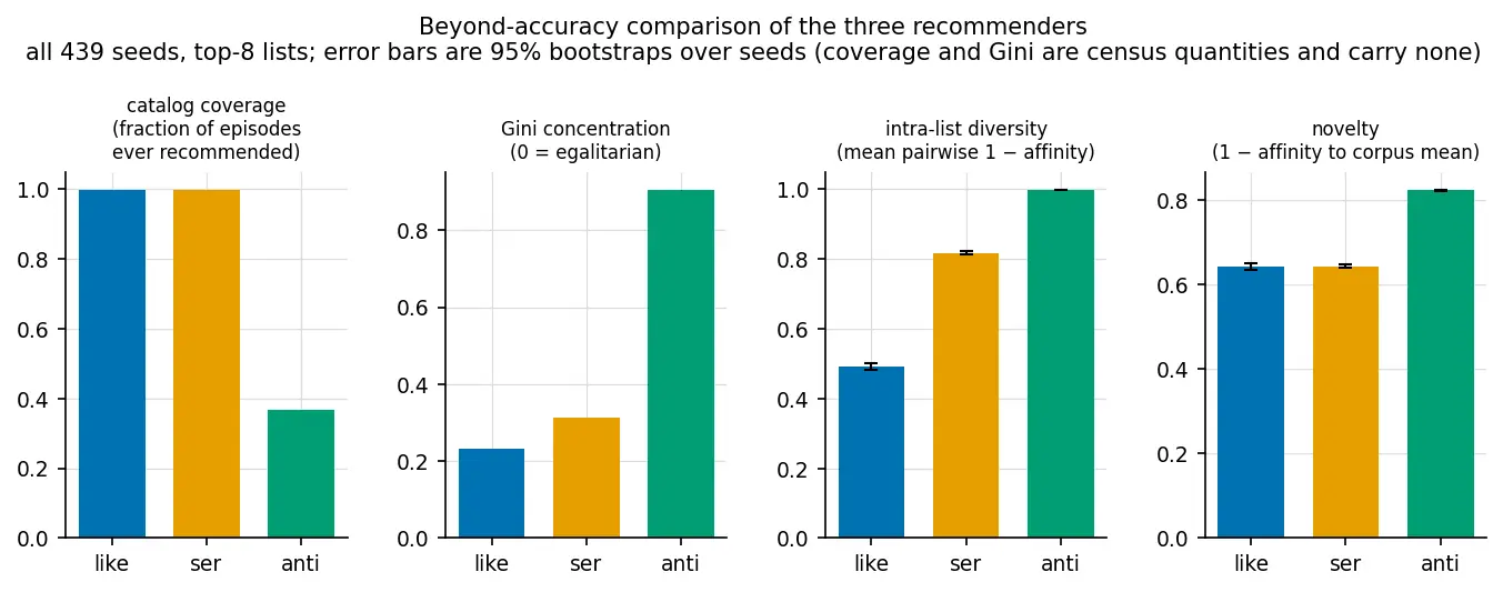
The lists are scored on the beyond-accuracy suite of Kaminskas and Bridge, with percentile-bootstrap intervals over the 439 seed episodes. The obvious list is as narrow as you would expect, with an intra-list diversity of 0.49. The serendipity list reaches 0.82, a paired difference of +0.33 (0.32 to 0.34), while still covering 99.8% of the catalogue, and at no measurable cost in novelty (a difference of +0.001, with an interval from −0.007 to +0.008). The “least likely” list reaches only 37% of episodes, with a Gini concentration of 0.91, because the show has a few far corners and every seed points at the same ones. That last number reassures me about the other two. The far corners exist, and the serendipity list is not simply sending everyone there.
Subjects that no episode has joined
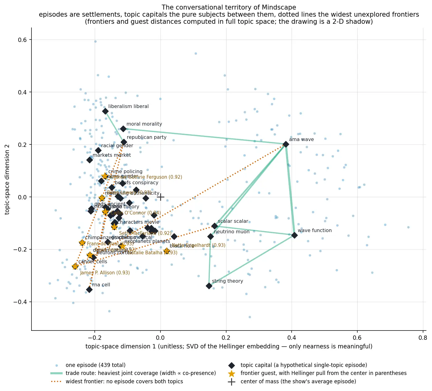
Think of the show as a map on which the well-visited subjects are cities and episodes are the roads between them. In the data, the co-presence of two topics is the sum over episodes of the smaller of their two shares, and among the show’s most-visited topics some pairs have almost none. The lowest is cancer and genetics with party politics and elections, followed by cancer and genetics with scalar fields, and the AMA cluster of wave functions and black holes with cancer and genetics. For each such gap the pipeline names the past guest whose own topic mix sits closest to both sides (Andrew Leigh, for the first pair) and the two specialists who could be invited together (James P. Allison with Ezra Klein). I do not imagine Sean books guests by consulting a co-presence matrix, but I enjoyed that the data can make a concrete suggestion.
A second representation
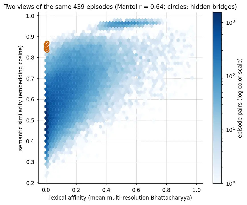
Everything so far is built from word counts, and a change of representation could change any of the answers. So the pipeline’s one model-inference stage encodes 33,522 passages of about 220 words, and 49,760 interview turns, with a sentence-embedding model (Qwen3-Embedding-0.6B), and then repeats the main analyses in that space. The two representations agree without being the same. The Mantel correlation between the lexical and semantic episode distances is 0.644 (p = 0.0005 over 2,000 permutations), and on average 46% of an episode’s ten nearest neighbours are shared between the two. The disagreements are the interesting cases, and the site lists them as hidden bridges (episodes that are close in meaning but share little vocabulary) and vocabulary collisions (the reverse). A few smaller findings hold in both spaces. Guests echo Sean’s words more than he echoes theirs in 85% of interviews, and the concepts whose contexts have drifted most across the show’s three epochs are “emergence”, “intelligence”, and “complexity”, with the semantic and lexical drift rankings agreeing at ρ = 0.75.
Searching by what you meant
The last thing I built is the one I use most. The Search page takes a question in plain words and returns the moments in the archive closest to what was meant, each with its timestamp, its speakers, the part of the passage that carries the query’s words, and a link to the episode. The engine is the relevance floor from Heart of Gold, a retrieval system I built earlier for Claude agents. A dense cosine pass over 20,842 transcript chunks gives a pool, a lexical channel adds any chunk containing the query’s rare words so that names and jargon are never lost, and a cross-encoder reranker reads each candidate against the query and gives a probability that it answers.
The reranker is the expensive part. It scores about 32 chunks a second on my machine, and the candidate pool is 376 dense chunks plus up to 376 lexical additions, so a full floor takes 12 to 24 seconds. Instead of guessing at an interactive budget, I measured what each budget keeps, against the fully reranked floor as the reference, over a set of blind queries.
| budget | share of the 28-chunk floor kept | share of the top 10 kept | wall time (median) |
|---|---|---|---|
| 4 s | 0.54 | 0.53 | 6.0 s |
| 6 s | 0.69 | 0.73 | 8.1 s |
| 8 s | 0.75 | 0.79 | 8.4 s |
| 12 s | 0.99 | 0.99 | 14.0 s |
The budget covers the reranker alone. Wall time also includes embedding the query, the dense pass, the lexical lookup, and whichever batch of 64 candidates the reranker was in the middle of when the deadline passed, which is why every row’s wall time runs past its budget. The service now runs at 12 seconds, which returns the full floor on nearly every query, and the page hides the wait by asking twice. The cosine-only floor comes back in about a second and is shown at once with a note, and the reranked list replaces it when it arrives. The whole thing runs on a Mac in my office through a Cloudflare tunnel, which is not how one would host a product, so when that machine is asleep the same search box falls back to a keyword index over the same passages and says so.
The companion page
The AMA checker is simpler than the search and has the cleanest evaluation of anything here. Sean’s show notes name who asked each listener question, so the 63 AMA episodes yield 2,581 question-and-answer pairs with their source known. The page embeds the questions and matches a new one against all of them, with no language model in the loop, so it answers in about 150 milliseconds and cannot invent anything. Because every harvested question is, by construction, already answered, the corpus is its own test set. On 200 questions submitted verbatim the right prior question ranks first every time. On 50 paraphrases it ranks first 98% of the time and within the top five always, with a worst rank of 2. The nearest other question sits at a median cosine of 0.635, which leaves room for the “close variant” band the page reports between an exact hit and a miss.
The transcripts are Sean’s
The site quotes only short passages, each with a link to its episode, and reproduces no transcript. The transcripts were collected from the site’s public API, respectfully and only a few times, and I have told Sean the work exists and offered to change or take down anything he would prefer not to see. That seemed like the least I owed someone whose eight years of conversations made the whole exercise possible.
If you have a question about the show that the search cannot answer, or you are working on something adjacent, I would be glad to hear from you.